Here is the link to my code. Note that you will need to install this open-source FLORIS python package from the National Renewable Energy Laboratory (NREL).
Recurrent Neural Network Architectures
In this project, we apply a number of different recurrent neural network architectures to the problem of forecasting the effective rotor-averaged wind velocity at 6 downstream wind turbines in a 3×3 wind farm in 1 minute intervals over a future 60 second horizon, given the turbine yaw angles, turbine effective rotor-averaged wind velocity and freestream wind speed components from the past 60 seconds in 1 second intervals. These include:
- Multi-Step LSTM
- Multi-Step GRU
- Autoregressive LSTM
- Autoregressive GRU
- Autoregressive Residual LSTM
- Autoregressive Residual GRU
Recurrent Neural Networks (Rnn)
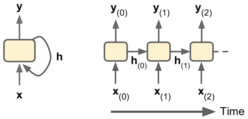
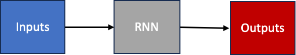
A recurrent neural network (RNN) describe a family of neural networks that are capable of handling sequential data, which for our purposes is time-series data. They consist of recurrent neurone which feed their output back into themselves as inputs. The figure below illustrates a simple RNN, consisting of a single recurrent neuron. On the left we see the condensed illustration, and on the right we see the unrolled representation. At each time-step, signified by the subscript on the variables below, a recurrent neutron receives the input from time step t, x_{(t)} and the previous state, h_{(t-1)}, as inputs and outputs y_{(t)}. This recurrent neuron has weights corresponding to each feature in x_{(t)} and h_{(t-1)} as well as a bias value, and includes an activation function.
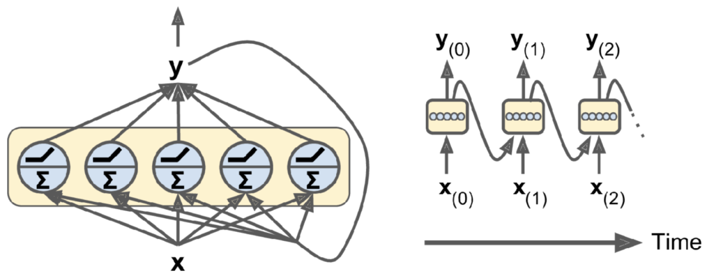
This simplified RNN can be expanded to consist of a layer of recurrent neurons, all of which receive the inputs, x_{(t)}, and previous state, h_{(t-1)} as illustrated in the figure below. On the left side of the image we see the condensed network. The \Sigma symbol represents the internal weighted sum operation within the neuron, and the ReLu function symbol represents the corresponding activation function for each neuron. On the right side we see the unrolled network, where in this case the ‘states’, h are equivalent to the outputs, y, and so are fed back into the recurrent layer.
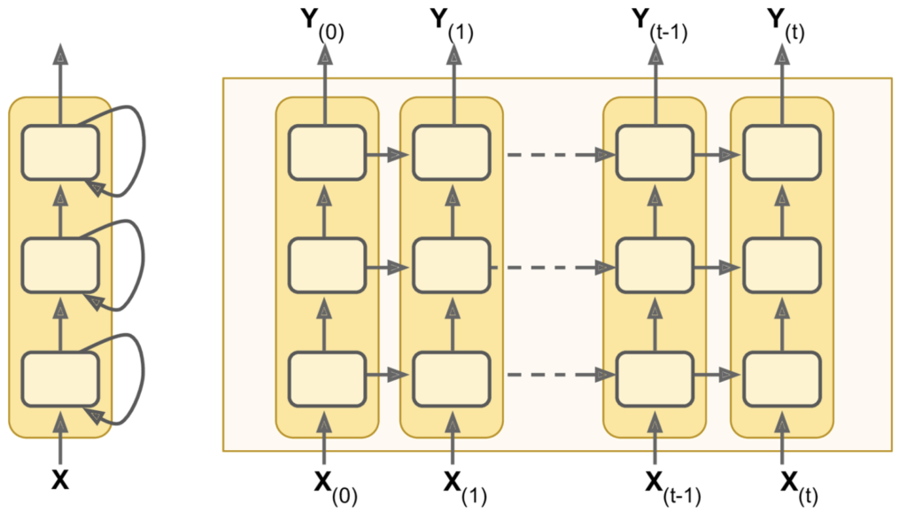
The next evolution of RNNs is generated by stacking recurrent layers in a deep recurrent neural network, illustrated below:
Note that we can choose our outputs, y, based on what it is we want to predict. In the case of time-series forecasting, if we wish to predict a particular feature or multiple features over a given future time-horizon (i.e. one step ahead of the inputs or multiple steps ahead of the inputs), we just change the training and test outputs to represent these target values. See the ‘Data Windowing’ section on the ‘Data & Preprocessing’ page for a review of how to do this.
long short term memory (lstm) networks
The Long-Short-Term-Memory cell was proposed to tackle the vanishing gradient problem observed in vanilla RNNs. It detects long-term trends in the sequential data.
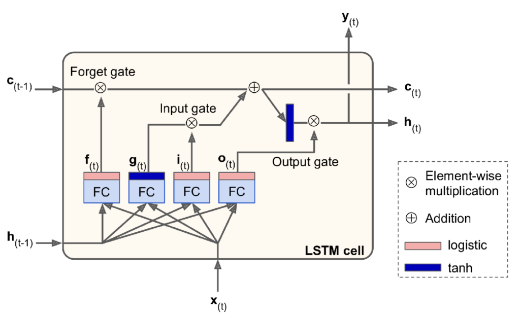
where h_{(t)} is the ‘short-term state’, c_{(t)} is the ‘long-term state’, and x_{(t)} is the current input vector. The purpose of the forget gate is to control which part of the long-term state is erased by multiplying it by f_{(t)} . g_{(t)} is the output of a layer that reads the previous short-term state and current input as inputs. The purpose of the input gate is to control what proportion of g_{(t)} is added to the long-term state. The purpose of the output gate is to control what proportion of the long-term state should be included in the output, y_{(t)}, and short-term state, h_{(t)}. Note that the g_{(t)} layer is activated by the tanh function such that unstable weights are saturated, and the other gate controller layers (outputting f_{(t)}, i_{(t)} and o_{(t)}) are activated by a non-saturating function such as the sigmoid.
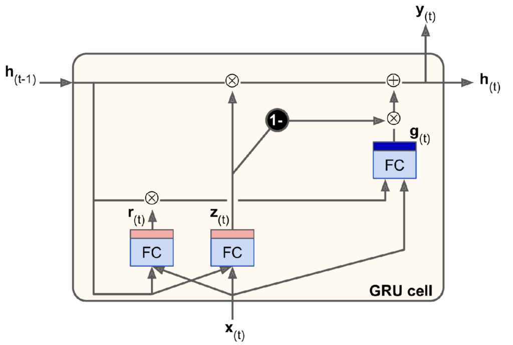
Gated Recurrent unit (Gru) Networks
The gated recurrent unit (GRU) cell illustrated below is a simplified variant of the LSTM cell described above. Compared to the LSTM cell: a) the long- and short-term states are merged into a single ‘hidden’ state, h_{(t)}, b) the forget and input gate controllers are merged into a single ‘update’ gate controller that outputs z_{(t)}, where a value of 1 results in the full previous state being passed on to the current and an output of 0 results in all of g_{(t)} being passed on, and c) instead of an output gate there is a new ‘reset’ gate controller that outputs r_{(t)} to control how much of the previous hidden state, h_{(t-1)}, is fed to the main layer that outputs g_{(t)}.
Multi-Step vs. autoregressive Output
Our goal is to make time-series predictions for multiple future time-steps given data from previous time-steps. There are multiple ways to achieve this, but in this project we implement two:
- Multi-Step Approach: Train the model to predict the set of future outputs at every time-step in a single prediction.
- Autoregressive Approach: Train the model to predict the outputs for a single future time-step, then feed that result back into the model inputs to generate the output for the next time-step.
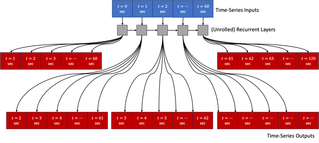
Multi-Step Approach
With this approach, we train a neural network to predict the next 60 seconds of output vectors at each input time-step (also 60 seconds worth in this case). This way, the loss function includes a term for the RNN output at every time-step, and so there will be many more error gradients propagating both through time and also through the model outputs. Ideally, this will stabilize and speed up the training process. We adapt the loss and metric functions to only consider the output from the last time-step, as these are the values used for prediction. We use the TimeDistributed layer to apply the Dense layer to every time-step, which in turn contains a cell for every future time-step prediction and every element of the output vector. We also need the series of a Reshape layer and Lambda layer, which add no tunable weights or biases, but rather transform the flattened outputs of the TimeDistributed layer back to (batch, time, features) from the predictions made at the last time-step. See an illustration of this architecture and the associated code below.
# Multi-Step LSTM RNN
models['multi_lstm'] = Sequential([
			LSTM(32, return_sequences=True, input_shape=[None, len(input_columns)]),
			LSTM(32, return_sequences=True),
			TimeDistributed(Dense(
				len(data_obj.input_columns) * int(data_obj.output_width // data_obj.output_step))),
			Reshape((int(data_obj.input_width // data_obj.input_step),
			         int(data_obj.output_width // data_obj.output_step),
			         len(data_obj.input_columns))),
			Lambda(lambda x: x[:, :, :,
		                 data_obj.input_columns.index(data_obj.output_columns[0]):(data_obj.input_columns.index(data_obj.output_columns[-1]) + 1)]),
			Reshape((int(data_obj.input_width // data_obj.input_step) *
			         int(data_obj.output_width // data_obj.output_step),
		         len(data_obj.output_columns)))
		])

# Multi-Step GRU RNN
models['multi_gru'] = Sequential([
			GRU(32, return_sequences=True, input_shape=[None, len(input_columns)]),
			GRU(32, return_sequences=True),
			TimeDistributed(Dense(
				len(data_obj.input_columns) * int(data_obj.output_width // data_obj.output_step))),
			Reshape((int(data_obj.input_width // data_obj.input_step),
			         int(data_obj.output_width // data_obj.output_step),
			         len(data_obj.input_columns))),
			Lambda(lambda x: x[:, :, :,
			                 data_obj.input_columns.index(data_obj.output_columns[0]):(
					                 data_obj.input_columns.index(data_obj.output_columns[-1]) + 1)]),
			Reshape((int(data_obj.input_width // data_obj.input_step) *
			         int(data_obj.output_width // data_obj.output_step),
			         len(data_obj.output_columns)))
		])

# Custom Loss Functions
def LastTimeStep_MeanSquaredError(y_train, y_pred):
	return mean_squared_error(y_train[:, -1, -1, :], y_pred[:, -1, :])

def LastTimeStep_MeanAbsolutePercentageError(y_train, y_pred):
	return mean_absolute_percentage_error(y_train[:, -1, -1, :], y_pred[:, -1, :])
autoregressive Approach
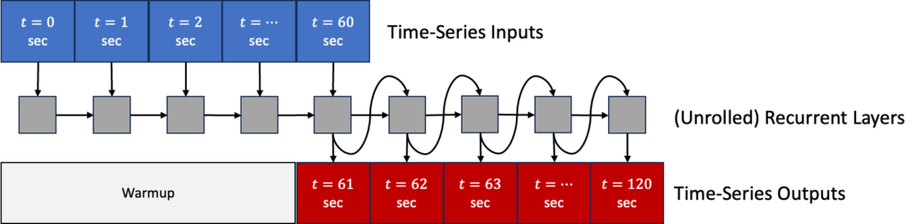
With this approach, we allow a ‘warmup’ period of training. We design a custom Feedback(Model) class that consists of a) either a LSTM layer (RNN(LSTMCell)) or a GRU layer (RNN(GRUCell)), b) a fully-connected layer (Dense), and c) a reshaping layer to reduce the vector of all predicted features to just those we care about i.e the effective rotor-averaged wind velocity at downstream turbines. We need layer c) because the features in the output of the dense layer must match the features in the inputs such that it can be fed back into the model to make predictions for the next time-step. We implement this layer with the Lambda custom layer class. In the custom class below, the ‘reshaping’ is only applied to the final outputs in y_preds, not to the outputs that are fed back into the model for each time-step. See an illustration of this architecture and the associated code below.
class Feedback(Model):
	def __init__(self, units, out_steps, num_features, cell_class, output_indices):
		super().__init__()
		self.out_steps = out_steps
		self.output_indices = output_indices
		self.units = units
		self.cell = cell_class(units)
		self.rnn = RNN(self.cell, return_state=True)
		self.dense = Dense(num_features)
		self.reshape = Lambda(lambda x: x[:, self.output_indices[0]:(self.output_indices[-1] + 1)])

	def warmup(self, inputs):
		x, *state = self.rnn(inputs)
		y_pred = self.dense(x)
		return y_pred, state

	def call(self, inputs, training=None):
		# tensor-array to capture dynamically unrolled outputs
		y_preds = []

		# initialize the LSTM state
		y_pred, state = self.warmup(inputs)

		# insert first prediction
		y_preds.append(self.reshape(y_pred))

		# run the rest of the prediction steps
		for i in range(1, self.out_steps):
			# use the last prediction as input
			x = y_pred

			# execute a single lstm step
			x, state = self.cell(x, states=state, training=training)

			# convert the lstm output to a prediction
			y_pred = self.dense(x)

			# add the prediction to the output
			y_preds.append(self.reshape(y_pred))

		y_preds = tf.stack(y_preds)
		y_preds = tf.transpose(y_preds, [1, 0, 2])
		return y_preds
Using the Feedback layer class, we can generate LSTM and GRU variants with 32 neurone in the RNN layers:
models['feedback_lstm'] = Feedback(units=32, out_steps=int(data_obj.output_width // data_obj.output_step), num_features=len(data_obj.input_columns), cell_class=LSTMCell, output_indices=[data_obj.input_columns.index(col) for col in data_obj.output_columns])

models['feedback_gru'] = Feedback(units=32, out_steps=int(data_obj.output_width // data_obj.output_step), num_features=len(data_obj.input_columns), cell_class=GRUCell, output_indices=[data_obj.input_columns.index(col) for col in data_obj.output_columns])
absolute vs. Residual predictions
Absolute Predictions
The final layer of all of the models codes above output a vector containing the effective rotor-averaged wind velocity at the downstream turbines, albeit normalized via the MinMax scaling as described in the ‘Data Normalization’ section on the ‘Data & Preprocessing’ page. We call these absolute predictions.
Residual Predictions
An alternative to the above is to design a neural network architecture with a final layer that outputs the predicted residuals to add to the outputs from the previous time-step to forecast the outputs at the next time-step. We call these residual predictions.
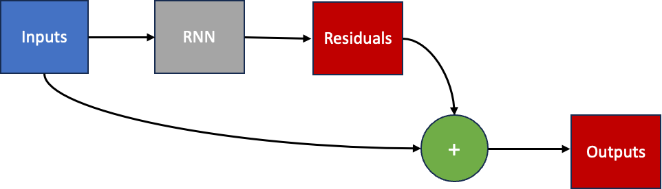
Below is a Residual model wrapper class that reads the output of the given model as a residual, selects the target values from the inputs passed to the model and adds them together to produce the new output.
class Residual(Model):
	"""
	This model makes predictions for each time-step using the input from the previous time-step
	plus the delta calcualte by the model.
	"""

	def __init__(self, model, output_indices):
		super().__init__()
		self.model = model
		self.output_indices = output_indices

	def call(self, inputs, *args, **kwargs):
		delta = self.model(inputs, *args, **kwargs)
		return inputs[:, :, self.output_indices[0]:(self.output_indices[-1] + 1)]  + delta
Using the Residual
models['multi_res_lstm'] = Residual(
		Sequential([
			LSTM(32, return_sequences=True, input_shape=[None, len(input_columns)]),
			LSTM(32, return_sequences=True),
			TimeDistributed(Dense(
				len(data_obj.input_columns) * int(data_obj.output_width // data_obj.output_step))),
			Reshape((int(data_obj.input_width // data_obj.input_step),
			         int(data_obj.output_width // data_obj.output_step),
			         len(data_obj.input_columns))),
			Lambda(lambda x: x[:, :, :,
			                 data_obj.input_columns.index(data_obj.output_columns[0]):(
					                 data_obj.input_columns.index(data_obj.output_columns[-1]) + 1)]),
			Reshape((int(data_obj.input_width // data_obj.input_step) *
			         int(data_obj.output_width // data_obj.output_step),
			         len(data_obj.output_columns)))
		]), output_indices=[data_obj.input_columns.index(col) for col in data_obj.output_columns] # indices of output columns in input columns
	)

models['multi_res_gru'] = Residual(
		Sequential([
			GRU(32, return_sequences=True, input_shape=[None, len(input_columns)]),
			GRU(32, return_sequences=True),
			TimeDistributed(Dense(
				len(data_obj.input_columns) * int(data_obj.output_width // data_obj.output_step))),
			Reshape((int(data_obj.input_width // data_obj.input_step),
			         int(data_obj.output_width // data_obj.output_step),
			         len(data_obj.input_columns))),
			Lambda(lambda x: x[:, :, :,
			                 data_obj.input_columns.index(data_obj.output_columns[0]):(
					                 data_obj.input_columns.index(data_obj.output_columns[-1]) + 1)]),
			Reshape((int(data_obj.input_width // data_obj.input_step) *
			         int(data_obj.output_width // data_obj.output_step),
			         len(data_obj.output_columns)))
		]), output_indices=[data_obj.input_columns.index(col) for col in data_obj.output_columns] # indices of output columns in input columns
	)
We write a similar wrapper class to handle models designed for auto-regressive approach called ResidualFeedback:
class ResidualFeedback(Model):
	def __init__(self, units, out_steps, num_features, cell_class, output_indices):
		super().__init__()
		self.out_steps = out_steps
		self.output_indices = output_indices
		self.units = units
		self.cell = cell_class(units)
		self.rnn = RNN(self.cell, return_state=True)
		self.dense = Dense(num_features, kernel_initializer=tf.initializers.zeros())
		self.reshape = Lambda(lambda x: x[:, self.output_indices[0]:(self.output_indices[-1] + 1)])

	def warmup(self, inputs):
		x, *state = self.rnn(inputs)
		delta = self.dense(x)

		# adding delta to last-time-step of each batch
		y_pred = inputs[:, -1, :] + delta

		return y_pred, state

	def call(self, inputs, training=None):
		# array to capture dynamically unrolled outputs
		y_preds = []

		# initialize the LSTM state
		y_pred, state = self.warmup(inputs)
		# insert first prediction

		y_preds.append(self.reshape(y_pred))

		# run the rest of the prediction steps
		for i in range(1, self.out_steps):
			# use the last prediction as input, should contain all features
			x = y_pred

			# execute a single lstm step
			x, state = self.cell(x, states=state, training=training)

			# convert the lstm output to a prediction
			delta = self.dense(x)

			y_pred = y_pred + delta

			# add the prediction to the output
			y_preds.append(self.reshape(y_pred))

		y_preds = tf.stack(y_preds)
		y_preds = tf.transpose(y_preds, [1, 0, 2])
		return y_preds
and similarly generate LSTM and GRU variants with 32 neurone in the RNN layers for the autoregressive approach:
models['feedback_res_lstm'] = ResidualFeedback(units=32,
out_steps=int(data_obj.output_width // data_obj.output_step),
num_features=len(data_obj.input_columns), cell_class=LSTMCell,
output_indices=[data_obj.input_columns.index(col) for col in data_obj.output_columns])

models['feedback_res_gru'] = ResidualFeedback(units=32,
out_steps=int(data_obj.output_width // data_obj.output_step),
num_features=len(data_obj.input_columns), cell_class=GRUCell,
output_indices=[data_obj.input_columns.index(col) for col in data_obj.output_columns])
Parameters-to-velocity transformation layer
An intended, secondary objective of this project was to use a recurrent neural network architecture to learn the parameters of a collection of analytical functions describing the wind velocity at the turbine locations in an online fashion, as the freestream wind speed and direction varies, and the nominal layout of the wind farm changes (i.e. due to one or more turbines temporarily ceasing to operate for repairs or due to a malfunction).
This layer requires not only the outputs of the previous stacked layers, which would be a vector of parameters rather than velocity values with this approach, but also a skip connection from the original inputs such that the layer knows what the current freestream wind speeds, freestream wind directions and turbine yaw angles are. Given these two distinct vectors, the layer can utilize FLORIS to update the parameterization of its internal analytical models and compute what the predicted effective rotor-averaged wind velocities would be for this parameterization.
There are two issues with this:
- We computed our ‘real’ training data with FLORIS, using the analyctical models for a given default parameterization, and now we are using FLORIS to compute our ‘analytical-model-predicted’ data. Ideally, we would use higher fidelity simulations as training data, but this was not possible given computational faculties available to the author. In any case, it is a good test of the parameter-tuning variation of this project to see if the neural network can converge to the default parameterization used in FLORIS to generate the training data.
- FLORIS is not tensor-friendly. It is a modular toolkit based on numpy arrays, and so little would be gained in terms of computational efficiency if this code were to run on GPUs, since tensors would need to be transferred to and from the CPUs for the tensor-to-array and array-to-tensor conversions.
Disclaimers aside, let’s look at how to achieve this anyway (as we are wont to do in academia). Below is a function to convert a merging of inputs (where the first element is the output of the preceding stackers layers – the parameters for the analytical models, and the second element is the set of training inputs fed to the first layer of the model). We transform it into a tensor-friendly function with the @tf.function decorator.
def numpy_params2pred(inputs, **kwargs):
	"""

	Args:
		inputs: vector of empirical gaussian parameters, bias term, freestreamWindVelX, freestreamWindVelY, yawAngles,

	Returns:

	"""
	params_input = inputs[0]
	training_input = inputs[1]

	config = dict(og_config)

	for model_type in TUNABLE_MODEL_TYPES:
		model_name = config['wake']['model_strings'][model_type]
		param_key = f'wake_{model_type.split("_")[0]}_parameters'
		list_idx = -1
		for param_name, idx in MODEL_TYPE_OUTPUT_MAPPING[model_type]:
			if type(config['wake'][param_key][model_name][param_name]) is list:
				list_idx += 1[list_idx], params_input[idx].numpy())
				config['wake'][param_key][model_name][param_name][list_idx] = params_input[idx]
				if list_idx == len(config['wake'][param_key][model_name][param_name]) - 1:
					list_idx = -1

	fi = wfct.floris_interface.FlorisInterface(config)

	freestream_wind_vel = tf.stack([training_input[:, :, input_columns.index("FreestreamWindSpeedsX")],
	                                training_input[:, :, input_columns.index("FreestreamWindSpeedsY")]], axis=-1)

	freestream_wind_vel = (freestream_wind_vel * (kwargs["data_max"][["FreestreamWindSpeedsX", "FreestreamWindSpeedsY"]]
	                                              - kwargs["data_min"][["FreestreamWindSpeedsX", "FreestreamWindSpeedsY"]])) \
	                      + kwargs["data_min"][["FreestreamWindSpeedsX", "FreestreamWindSpeedsY"]]

	freestream_ws = tf.norm(freestream_wind_vel, axis=-1)
	freestream_wd = tf.math.asin(-(freestream_wind_vel[:, :, 0] / freestream_ws)) * (180 / np.pi)
	y_preds = []
	for batch_idx in range(freestream_ws.shape[0]):
		time_step_idx = -1
		fi.reinitialize(wind_speeds=[freestream_ws[batch_idx, time_step_idx]],
		                wind_directions=[freestream_wd[batch_idx, time_step_idx]])
		yaw_angles = (np.array([training_input[batch_idx, time_step_idx, i] for i in yaw_angle_idx]) \
		              * (kwargs["data_max"][yaw_angle_cols] - kwargs["data_min"][yaw_angle_cols])
		              + kwargs["data_min"][yaw_angle_cols]).to_numpy()
		fi.calculate_wake(yaw_angles=yaw_angles[np.newaxis, np.newaxis, :])
		y_preds.append(fi.turbine_effective_velocities[0, 0, downstream_turbine_indices] + params_input[-1].numpy())
	return np.vstack(y_preds)


@tf.function
def tf_params2pred(inputs):
	return tf.numpy_function(numpy_params2pred, inputs, tf.float32)
With this function, we can create a custom Lambda layer, and create a LSTM with our parameter-to-velocity layer at the end:
Params2Pred_Layer = Lambda(lambda x: tf_params2pred, output_shape=(len(data_obj.output_columns),))

input_layer = Input(shape=data_obj.train.element_spec[0].shape[1:])
models['pred_lstm'] = LSTM(32, return_sequences=False)(input_layer)
models['pred_lstm'] = Dense(units=(N_PARAMS + 1))(models['pred_lstm'])
models['pred_lstm'] = Params2Pred_Layer([models['pred_lstm'], input_layer])
models['pred_lstm'] = Model(input_layer, models['pred_lstm'])
That concludes the description of the deep learning methods employed in this project. Now, on to the results!