Aoife Henry

Raw Data

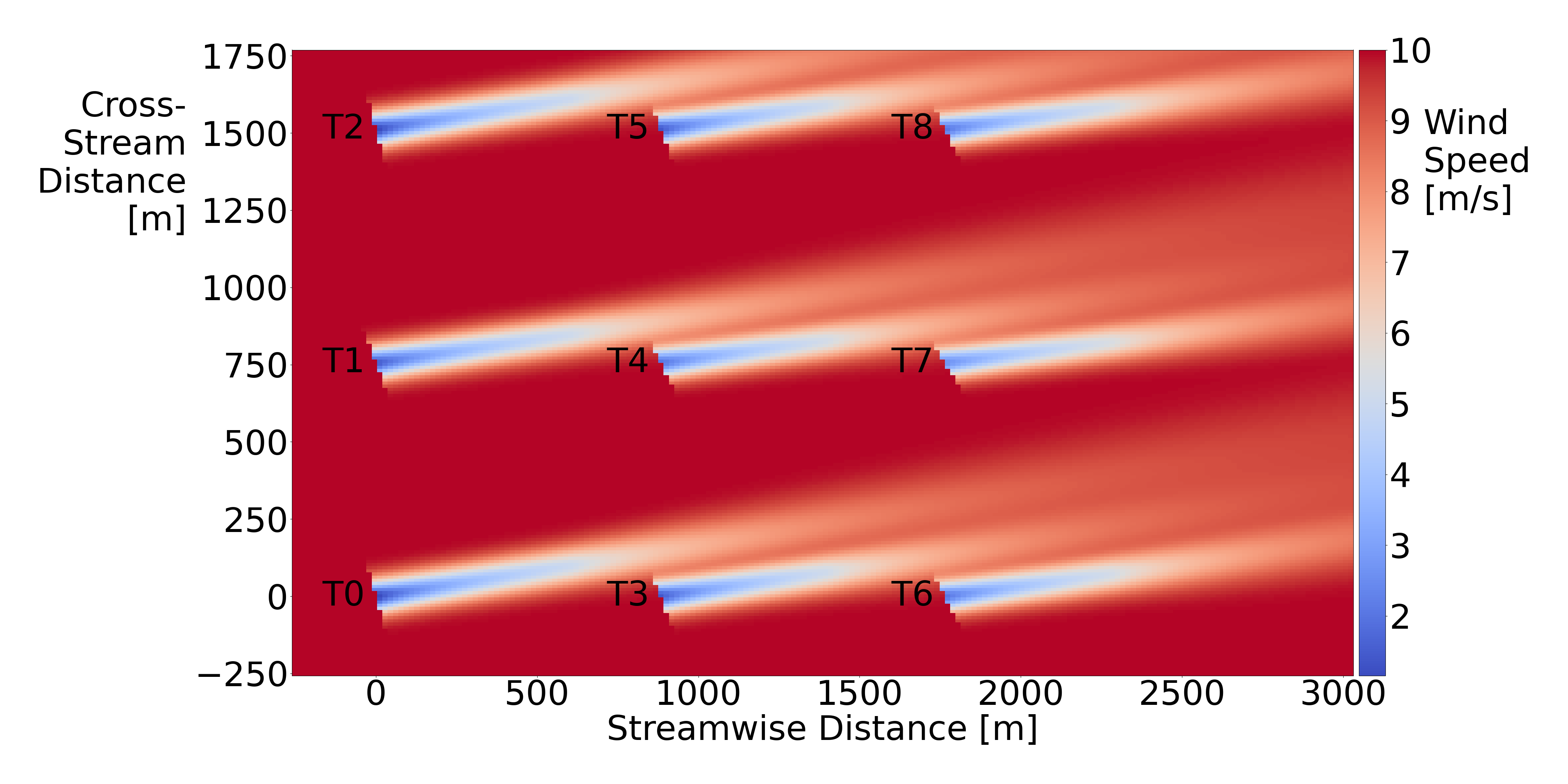
The goal of this project is to predict the effective rotor-averaged wind velocity (the component of the wind velocity that is perpendicular to the wind turbine, averaged over several points over the area spanned by the blades) at downstream wind turbines in a wind farm over a given future prediction horizon. Downstream wind turbines refer to those that lie in the wake of other, upstream wind turbines in the farm. In the figure below; T0-T5 would be considered upstream turbines, whereas T3-T8 would be considered downstream turbines. The astute reader will note that these categories do indeed intersect – the middle ‘row’ of turbines, T3-T5, are included in both.

The raw time-series data consists of ten, 3600 second (1 hour), low-fidelity simulations of a wind farm (using the open-source NREL software FLORIS) given time-varying freestream wind speed and direction and time-varying yaw angles for each of the wind turbines. Freestream wind refers to the average speed and direction of the wind outside of the wind farm (where it is not perturbed by any pesky turbines). The yaw angles refer to the rotational position of each turbine about a vertical axis.

The WakeField.py file contains all of the code necessary to generate the data, given that the FLORIS module is installed. It generates time-varying sequences of baseline mean values of freestream wind speed, freestream wind direction, and yaw angles (for each of the turbines in the 3×3 wind farm). These values are first randomly initialized within an allowable range of values (given by the mean value range shown below). Then, for each sampling time of 1 second, there is a nonzero probability, given by the probability of mean value change number below, that the mean values will be incremented or decremented by the change to mean value numbers below. Once we have the new, or unchanged mean values, Gaussian noise with zero mean and standard deviation given by the standard deviation of Gaussian noise number below is added to the mean values. The parameters used to compute these sequences are as follows:

• Freestream Wind Speed
  • Mean values between 8 and 16 m/s
  • Probability of mean value change is 0.1
  • Change to mean value if it does is 0.5 m/s
  • Standard deviation of Gaussian noise added to mean is 0.5 m/s
• Freestream Wind Direction
  • Mean values between 250^\circ (corresponds to a south-westerly wind direction, as in figure above) and 270^\circ (corresponds to a westerly wind direction)
  • Probability of mean value change is 0.1
  • Change to mean value if it does is 5^\circ
  • Standard deviation of Gaussian noise added to mean is 5^\circ
• Yaw Angles
  • Mean values between -30^\circ and 30^\circ
  • Probability of mean value change is 0.5
  • Change to mean value if it does is 30^\circ
  • Standard deviation of Gaussian noise added to mean is 0^\circ

Given the freestream wind speed, freestream wind direction and yaw angles of each wind turbine, we use FLORIS to compute the effective rotor-averaged wind velocity at each downstream wind turbine and add these to the dataset.

Ten such 3600 second time-series datasets are simulated in this fashion, linked here in CSV format, which are then ready for pre-processing.

Note that in the original data, the freestream wind data is given as a pair of absolute wind magnitude in m/s and wind direction in degrees for each time-step. The freestream wind speed components in the s , and c , directions need to be computed from the wind magnitude and direction available in the raw data, since the cyclical nature of directional angle measurement in degrees (i..e. the equivalence of 0 degrees and 360 degrees) is not rational for a neural network architecture. We do this with the following code, where FreestreamWindSpeedsX is equivalent to the streamwise direction and FreestreamWindSpeedsY is equivalent to the cross-stream direction.

			# get freestream wind speed data
                        wind_speeds = df.pop('FreestreamWindSpeed')
	                
                        # get freestream wind direction data and convert to radians
			wind_directions = df.pop('FreestreamWindDir') * np.pi / 180

			# compute freestream wind speed components where 0 deg = (from) northerly wind,
			# 90 deg (from) easterly, 180 deg (from) southerly and 270 deg (from) westerly
                        df[f'FreestreamWindSpeedsX'] = wind_speeds * -np.sin(wind_directions)
			df[f'FreestreamWindSpeedsY'] = wind_speeds * -np.cos(wind_directions)

The first few rows of this dataset, in a pandas.DataFrame form, are shown below. Note that some unnecessary data included in the raw data is not included.

>>> wf_dfs[0][[col for col in wf_dfs[0].columns if 'AxIndFactors' not in col and 'Time' not in col]].head().transpose().sort_index()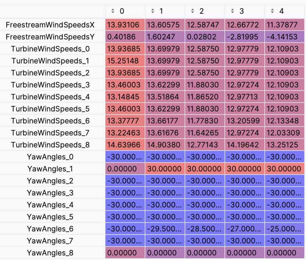

Below we have all of the relevant features in the raw datasets. FreestreamWindSpeedsX and FreestreamWindSpeedsY refer to the streamwise (s) and cross-stream (c) freestream wind speed components, respectively. TurbineWindSpeeds_x refers to the effective rotor-averaged wind velocity at the xth wind turbine (zero-indexed) and YawAngles_x refers to the yaw angle setpoint of the xth wind turbine.

>>> sorted([col for col in wf_dfs[0].columns if 'AxIndFactors' not in col])
['FreestreamWindSpeedsX', 'FreestreamWindSpeedsY',
 'Time',
 'TurbineWindSpeeds_0', 'TurbineWindSpeeds_1', 'TurbineWindSpeeds_2',
 'TurbineWindSpeeds_3', 'TurbineWindSpeeds_4', 'TurbineWindSpeeds_5',
 'TurbineWindSpeeds_6', 'TurbineWindSpeeds_7', 'TurbineWindSpeeds_8',
 'YawAngles_0', 'YawAngles_1', 'YawAngles_2',
 'YawAngles_3', 'YawAngles_4', 'YawAngles_5',
 'YawAngles_6', 'YawAngles_7', 'YawAngles_8']

possible targets/Outputs

Effective Rotor-averaged wind velocity at each turbine

The rotor of a wind turbine refers to the area spanned by its (normally) three blades, upon which the wind is incident. The rotor-averaged wind velocity at a wind turbine is computed by measuring the velocity at several points across the rotor area and averaging them. This effective transormation of this measurement is computed by considering the misalignment between the direction the rotor is facing (as determined by the yaw angle) and the current wind direction, and projecting the absolute wind velocity onto the axis perpendicular with the rotor..

Parameters for analytical models describing rotor effective wind velocity at each turbine

A subject for future work (read: try as I might I couldn’t convince Tensorflow to work with me within the time constraints of this project) involves using RNNs to learn time-varying parameters for a combination of analytical models describing the wind field inside a wind farm in an online fashion. These models include a) the empirical Gaussian model for describing wake velocity deficit at downstream wind turbines, b) the empirical Gaussian model for describing wake deflections at downstream wind turbines, and c) the wake induced mixing model for describing the turbulence intensity in the wakes incident on downstream wind turbines.

The logic for tuning the parameters of these models online is that the best-fitting parameterizations for the models are likely to change with changing wind direction and on the occasions where one or more turbines are not operational. In particular, the latter case is true upwards of 90% of the time, even though these models are tuned on the assumption of a fully operational wind farm. Given a more accurately parameterized description of the wind farm dynamics, such a model could be included in a model-based receding horizon controller, such as model predictive control (MPC), to optimally control the yaw angles of the wind turbines over a future time horizon.

Implementing a deep learning algorithm to learn the parameters of analytical models is not trivial. Our output labels are in the form of effective rotor-averaged wind velocities at downstream turbines, not parameters. It is these wind velocity values that must be ultimately output from the model in order to compute the loss function values. We therefore require a Lambda layer in Tensorflow – a custom layer with no learned parameters to transform the output of the preceding stacked network layers (the parameters) into wind velocities predicted by the combination of analytical models for these parameters.

Inputs & Outputs

The inputs, X , consist of the freestream wind speed components in the streamwise (s) and cross-stream (c) coordinates (see figure above), the yaw angles of all wind turbines, and the measured effective rotor-averaged wind velocity at all upstream wind turbines. The output labels, y , consist of vectors of the effective rotor-averaged wind velocity at all 6 downstream wind turbines.

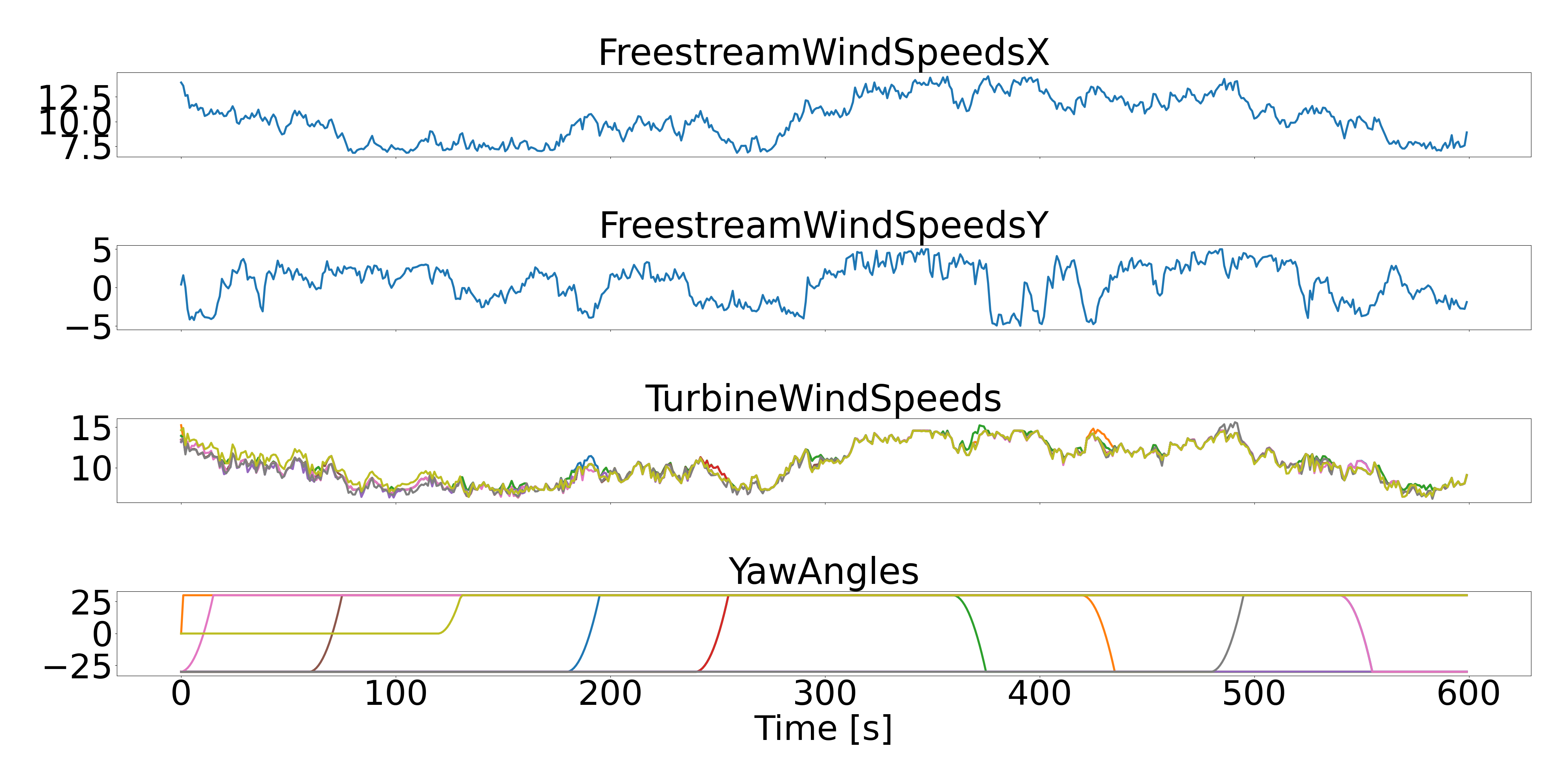
Below are plots of a 10 minute subset of the first training dataset features. Note that the different colours in the third TurbineWindSpeeds and fourth YawAngles plots correspond to each of the nine wind turbines in the farm.

Data Normalization & division

The MinMax transformation is used to normalize the data to values between 0 and 1: \tilde{X} = \frac{X – \underline{X}}{\overline{X} – \underline{X}}

where \underline{X}, \overline{X} represent the minimum and maximum values of each feature of the input matrix, X , respectively.

Once the time-series data has been normalized, the ten 1 hour simulations are divided between training (70% – 7 simulations), validation (20% – 2 simulations) and testing datasets (10% – 1 simulation).

Below are statistics describing the first of the normalized training datasets::

>>> train_dfs[0][[col for col in wf_dfs[0].columns if 'AxIndFactors' not in col and 'Time' not in col]].describe().transpose().sort_index()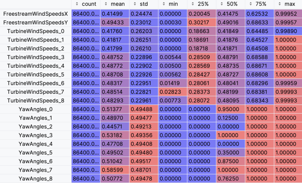

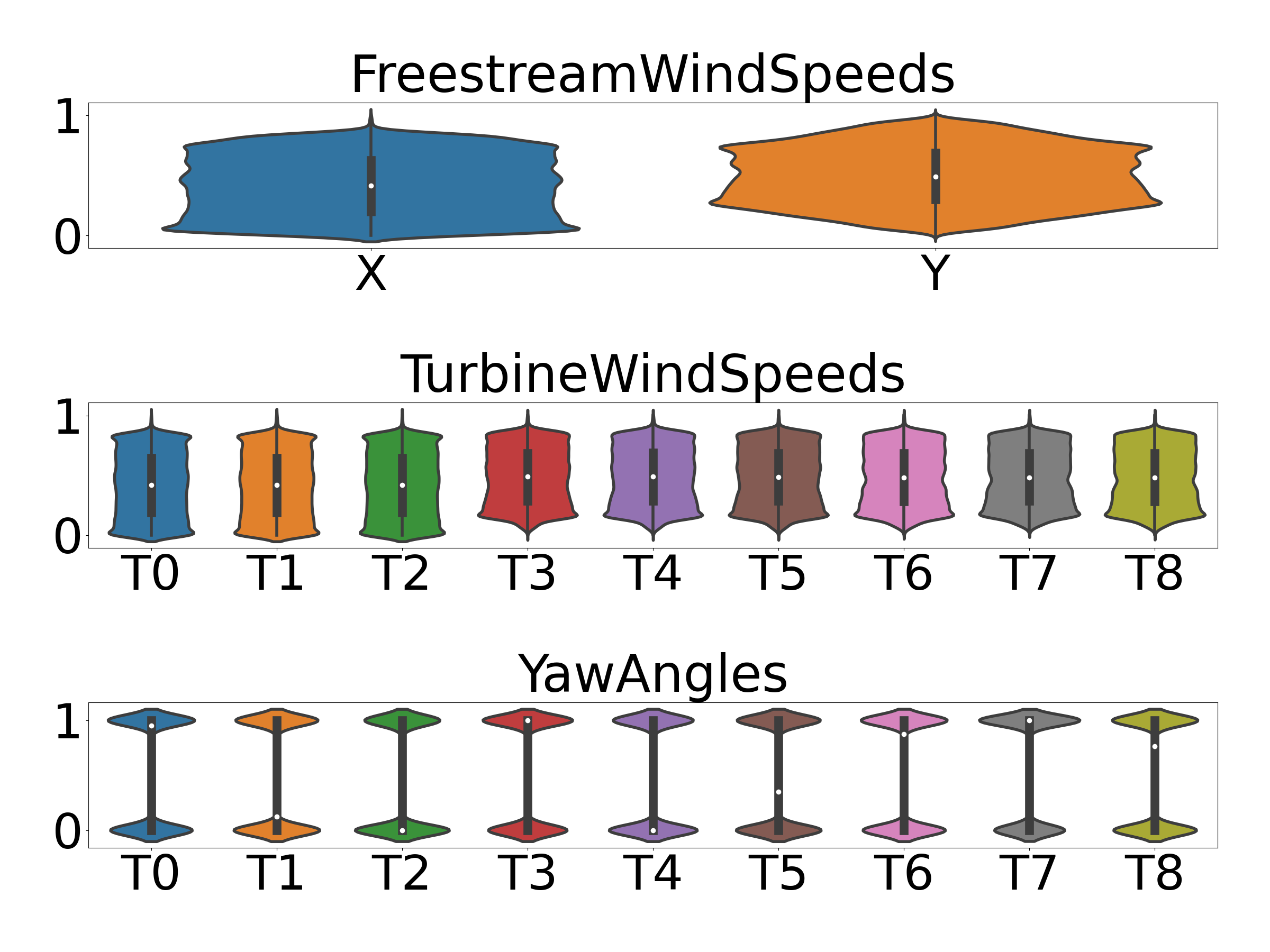
Once normalized to values between 0 and 1, we can inspect the distribution of the values with a violin plot. The top plot shows the streamwise (s) and cross-stream (c) components of the freestream wind speed (X and Y in the plot below), the middle plot shows the effective rotor-averaged wind velocity for each of nine turbines, and the bottom plot shows the yaw angle setpoints for each of the nine turbines. The width of the violin area for each vertical value correlates with the frequency of the data in that region. We see from the YawAngles plot, that much of the time the yaw angles are at their extreme values of 0 and 1 (equivalent to \pm 30^\circ and the relatively low frequency for intermediary values occur during transition between these extremes. We can also see from the FreestreamWindSpeeds plot that the streamwise component, FreestreamWindSpeedsX, is more evenly distributed than its cross-stream counterpart, FreestreamWindSpeedsY. There also appears to be a pattern of more uniform effective rotor-averaged wind velocities at extreme values for the most upstream wind turbines (T0, T1 and T2), as compared with the more downstream wind turbines (T3 – T8).

The normalized and divided data can be found here in pickle format as a list of training, testing and validation time-series datasets.

Data Windowing

This is a time-series forecasting problem, in which we want to predict the effective rotor-averaged wind velocities at downstream turbines over a future time horizon of 60 seconds at 1 second intervals, given the inputs received over the last 60 seconds at 1 second intervals. We thus format the inputs and labels suitably for a time-series forecasting algorithm that predicts several steps ahead given inputs from several steps before. This involves generating data batches of 64 samples of time-series data spanning a full time-window of 2 minutes from each 1 hour simulation and splitting the data into inputs, X, corresponding to the first 60 seconds, and output labels, y, corresponding to the last 60 seconds. The data batches from all 10 simulations are then concatenated together and shuffled.

To this end we write a Data class in the Data.py file with make_dataset and split_window methods, where the former generates batches of time-series data and the latter splits it into suitable time-windows.

Now, the original time-series data has a) been transformed and normalized appropriately, b) divided between training (70%), validation (20%) and testing datasets (10%), c) been split into batches of time-series’, and d) been split into input and output data. Below is a representation of the resulting training dataset shapes.

All shapes are: (batch, time, features)
Inputs shape (batch, time, features): (64, 60, 20)
Labels shape (batch, time, features): (64, 60, 6)

For some of the models (namely, the multi-step prediction approach, described in the next section) implemented, we require a sequence of labels predictions for each input time-step, in which case the training dataset has the following shapes:

Input shapes are: (batch, input_time, features)
Inputs shape (batch, input_time, features): (64, 60, 20)

Output shapes are: (batch, input_time, output_time, features)
Labels shape (batch, input_time, output_time, features): (64, 60, 60, 6)

Now that we have transformed, normalized and suitably formatted input and output data, divided into training, validation, and test datasets, we are ready to use this data with recurrent neural network architectures, described next.